Stackmatch Initial Tests

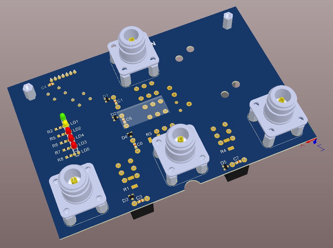
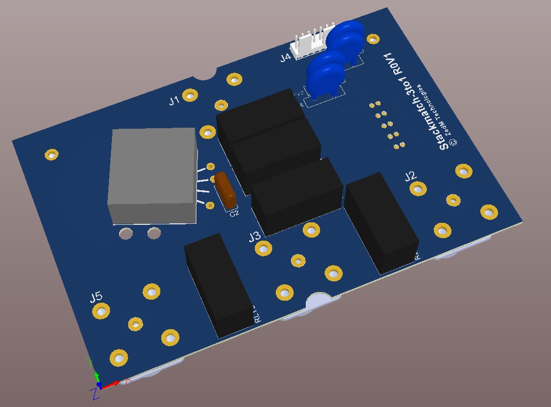
Well the Stackmatch PCB’s finally came back from the Manufacturer along with the components from Mouser, so it was time to build.  I’m pleased with the 3D model and the actual final assembly, they are pretty close !

This slideshow requires JavaScript.

I’ve not mounted the LED’s on the left hand side yet, this will wait until I can drill the front panel of the diecast enclosure and begin final assembly.  Since I’ve got more than one of these to make I’m getting a template made from steel that I can mount on the front panel and then drill all the holes.

The assembly in the picture above is the first prototype and I wasn’t going to wait for the front panel and die-cast box to be ready before testing.  The connectors have been attached at roughly the right height using an additional nut as a spacer, I’ve only fitted half the standoffs to save some time.

So the question is does it work?

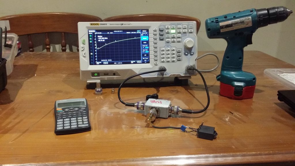
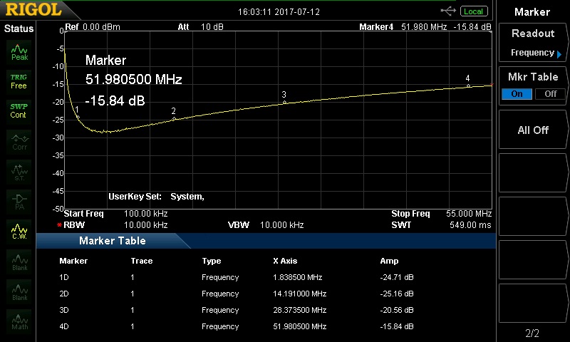
The first test is simply a test of the isolation between ports.  So taking a spectrum analyser with tracking generator the idea is to measure the insertion loss between the input and one output as we switch between all three outputs one at a time and record the results.  All outputs are terminated in a 50 ohm load.  What is interesting with this stackmatch is we can also select “no outputs” where no relays are energised, this has a surprising result on the measured isolation;

This slideshow requires JavaScript.

OK, so what can we deduce from these series of plots.  The Spectrum analyser (SA) tracking generator was on the Stackmatch input, the SA input was on Output #1 unless you missed it.   As we switch each output from #1 to #3 we can see the insertion loss change.  As you would expect when we select output #1 we measure the insertion or through loss of the stackmatch, when we select any output other than #1 we measure the Isolation between ports.

Here’s the all important worst case summary, which is of course at the high end of the HF band i.e 10m;

  • Insertion Loss < -0.2dB
  • Isolation > 37dB

That is not too bad for a single device covering from 160m to 10m.  In real terms it means when we are transmitting 400W PEP (+56dBm) on 10m that less than 80mW (+19dBm) will be leaking out the other two ports.  The same can be said for helping prevent overload in the receiver from adjacent contest stations (i.e. on 20m).  The AREG typically use Elecraft K3’s and high end Icom transceivers so these typically don’t give too hoots about QRO contest stations on adjacent bands in the first place.     The best part is as we go lower in frequency the Isolation increases a further 10dB which can only improve the situation.

The insertion loss is barely measurable, so nothing should be getting really hot or require further bypassing.

Now what was also interesting is the difference in output isolation with no outputs being selected and just one.   The isolation to an unused port increased by +5dB to +6dB when the input was terminated into just one antenna.  That is something that we’ll need to take care of with our control system, not selecting any output is bad.

So then it was a question of moving the Spectrum Analyser input to Port #2, terminating Port #1 and repeating the above measurements again.  We do the same again for Port #3, shuffling the dummy loads and measuring once more.  I’ll not bother putting up all of these plots, suffice to say all of the isolation between ports were within 0.5dB of each other and insertion loss didn’t move.

Now for the main event, parallel combinations.

To do this we use a Return Loss (RL) measurement, so I’ve placed the RL bridge on the input to the Stackmatch and then terminated every output in a good quality dummy load, this is important !.  Then by switching the outputs in succession I can generate the various parallel combinations (25 ohms and 16.7 ohms) and then switch the transformer into to see the effect.  In all cases a 30pF Silver Mica cap has been tacked across the output of the auto transformer as per our previous experiment (click).  Here’s the measured plots;

This slideshow requires JavaScript.

So from our first plot where only one output is selected our return loss looks excellent with the minor exception of a spike at 8MHz.   I’m not sure that this is real just yet and will be doing some further work on what that resonance could be.  It’s got to be a parasitic capacitance there somewhere, will track that down later.   You might notice that the RL is better than -20dB (1.2:1) anyway, so a moot point really.

When we place output #1 and #2 in parallel we get 25 ohms and the RL rises to -10dB as you’d expect.  Then when we kick in the transformer we see an immediate improvement of RL to better than -18dB (1.3:1) at worst case (10m).

Now when we place all three outputs in parallel our RL is destroyed -6dB, but again if we kick in the transformer we see an improvement in RL of -13.5dB (1.6:1).  If you get your calculator out you find the ratios are smack bang on our design of 2.25:1.    So to summarise;

  • Return Loss (1-output) < -20dB
  • Return Loss (2-output) < -18dB
  • Return Loss (3-output) < -13dB

Yaay it works !

So there we have it, the beginnings of a workable stackmatch design.  As with any new design there is still plenty to be tweaked and played with.  In the coming weeks I’ll be;

  • investigating the effect of the cap across the output
  • chasing down that odd parasitic resonance at 8MHz with one antenna selected
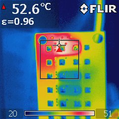
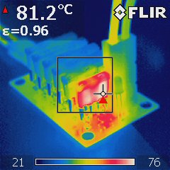
  • measuring the temperature rise of the transformer with 120W of CW being blasted into it, or 300W of RTTY to give it some real curry…
  • Making the final enclosures and seeing what effect (if any) this has on the design
  • Trying #16, #20 & #24 gauge PTFE wire on the same core to see if the performance or characteristics of the transformer changes
  • Seeing what effect the +/- J term from various antennas has on the combined feed point impedance that our radio will see (thanks to David VK5DGR for bringing that one up !)

Yes it’s going to be a busy few months as we explore what this new toy can do.

Stackmatch Binocular Matching Transformer

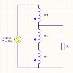
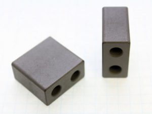
Many stackmatch designs use a toroid core, but I’ve decided to  instead investigate using a multi-aperture “binocular” core.

There are not many manufacturers of large-ish binocular cores that can take the full VK HF limit of 400W PEP, let alone a full kilowasp amplifier !

So to start with I’ve chosen two well known binocular cores that you can obtain from various online suppliers;

  • Amidon BN-61-002
  • Fair Rite 2861010002

Both are the equivalent of each other in terms of price, size and material.  Both are made from Type 61 NiZn Ferrite material with a ui of approximately 125.   This material has good low loss properties and is essentially what others have used for their toroid designs.  It seems like a good place to start.

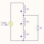
The transformer is wound the same way as if on a toroid, so take three wires, twist them together (battery drill helps) and wind the desired number of turns through the holes.   It seems sensible to start with a full core and take turns off if I achieved too much inductance.  Both of these cores hold ~4 turns of trifiliar wound 20AWG silver plated PTFE wire, it might add the last turn is hard to do.  All that is left is to series up the windings and tap at the appropriate positions, the schematic is to the right.

To make my measurements I decided to use a variable resistor (R1) to check the effect of load change on the transformer.  I had also seen some designs using a small amount of shunt C across the output to neutralise the output leakage inductance as well, so I placed a variable cap across the variable resistor when needed.

To make these measurements I’m fortunate to have a Spectrum Analyser with tracking generator and a suitable Return Loss Bridge.  The return loss bridge has a directivity of > 45dB at HF.  This means I can see how much energy is being transferred to the load resistor (R1), any RF energy that is being reflected back to the spectrum analyser is therefore wasted, so in all of the screen captures below the lower the Return Loss the better !

You can see the experimental setup in the image below and my initial measurement on the kitchen table…

I’d start these measurements by adjusting R1 until I achieved the lowest Return Loss and then remove the resistor temporarily and measure it separately with a 4-digit ohmmeter.  I wanted to check that I was close to 22.2 ohms in all cases.   With such a low resistance don’t forget to deduct the resistance of the multimeter leads.

Once I had confirmed the impedance transformation was correct I would then tack the trimmer cap across R1 and start with it completely un-meshed (min C).   The cap on the secondary side of our transformer will assist in “tuning” out the output reactance (Xs) of the transformer a little and improving the return loss at the upper end of our plot.

However there is a null that will occur at the low end of VHF that you need to be wary of as it can be unstable, you can if you have enough capacitance bring it into HF spectrum which is not advisable.   You will easily see the point where I’ve added too much in the sequence below.   What you’re looking for is just enough turns to give you the broadest match possible with the smallest value of C across it’s output.

Here’s a sequence of plots showning what happens as you increase C from min (5p) to too much (120p).  This was with 3 turns wound through the core, R1 approx 22.3 ohms;

This slideshow requires JavaScript.

So in the above sequence you can see what the effect that the capacitance has across the output.  As we keep adding capacitance the return loss kept getting better and better before the null appears.  The ideal compromise was somewhere between 65p-80p.

What you can also do is widen out the frequency from 1-200MHz and watch what effect any nulls will have on the response.  It also pays to vary the load (R1) and see what happens as the load decreases below and above the desired match.   I found that as the output impedance goes up the null has a much more prominent effect as the load is varied.

So starting at 4 turns I checked the impedance ratio and then wen’t looking for the best compromise in terms of response, stability and lowest capacitance.   Below are the three best candidates that I found;

This slideshow requires JavaScript.

So as we reduce the turns (inductance!) we see the return loss decrease at the low end, but we also see the required capacitance to flatten out the upper end also reduce.   Based on these measurements the best compromise I found for this transformer is 2T C=30p.   Ideally a return loss less than -20dB is a good target to aim for, I’ll let the reader work out what the equivalent VSWR is for this RL value (hint: it’s low, for additional points also take a look at a RL of -10dB for reference !).

Now to check that this is stable I’ve included a plot that is much wider in terms of checking the VHF region for signs of that null we wish to avoid.  Hmm, this combination is potentially usable up to 6m, now there’s an idea for another day.

Sweet no signs of the null being anywhere close to the MF/HF bands I want to operate over.

Now the ultimate test is to make two of these transformers, place them back to back into a 50 ohm load then measure the insertion loss. That will give me some idea on what sort of loss this transformer will have an ultimate how hot it will get when I attempt to pass 120W CW/FM or 400W pep of SSB.

More to come.

Yet Another Stackmatch Design

In October each year I join my local radio club AREG and participate in the Oceania DX (OCDX) contest.   For the past few years I’ve been the band captain for the 15m/10m station.  We started in 2014 with just an Icom IC-706mk2 and 2 element broadband Hexbeam, but this quickly morphed into a complete Elecraft K-line, Amplifier, SDR’s, filters and Spiderbeam on a 8m pump up mast; as a portable station.

This slideshow requires JavaScript.

So to take our station yet another step forward we need to add additional antennas like mono-band verticals to take advantage of lower propagation angles. Here in VK we are along way from anywhere, so the majority of our propagation on most bands is below 20 degrees.   However before you can take advantage of these additional antennas you need to switch between them.

Trolling the internet for inspiration we discovered the 3 to 1 Broadband Stackmatch.  This is a simple 3 port antenna switch that can individually switch each antenna to the radio, but it can also be used to parallel up any two or all three antennas ports together.

It exploits the fact that two 50+j0 ohm antennas in parallel is 25+j0 ohms and three in parallel just shy of 16.7+j0 ohms.  So by inserting a transformer with a fixed impedance matching ratio we can bring the parallel antennas effective impedance back up close enough for many amplifiers/transceivers not to care about the minor mismatch.   So that is deviously clever and simple.

The equivalent circuit of a stackmatch transformer is shown to the right, you’ll see it drawn many different ways but I find it easier to understand when drawn as an autotransformer.

Accordingly the maths says;

n = Np / Ns
Z’ = (n)^2 x Zload

So lets see what happens;

Np = 3, Ns = 2, n = 3/2 = 1.5

So with two antennas in parallel;

Z’ = (1.5)^2 x 25 = ~65.3 ohms

With three antennas in parallel;

Z’ = (1.5)^2 x 16.7 = ~37.6 ohms

This small impedance mismatch (~14 ohms) either side of 50 ohms will not cause many radios much difficultly. It does however tell us that we must ensure that our antennas are resonant (50+j0) since we have ignored the imaginary impedance for simplicity.  What is also not explained is you need to keep the feedlines to each antenna from the stackmatch as close to the same length as you can or there be more trouble with impedance transformations.

There are plenty of designs on the internet and products available from suppliers but their cost are quite simply prohibitive, especially if you want 6 or more of these units to achieve your desired switching arrangement (*gasp*) at a contest.

So here starts yet another project to design and build my own low cost 3 to 1 Stackmatch.   It certainly has not taken long to come up with a workable 3D model.  It kind of helps that I design products like this every day as an Design Engineer.  I’ve also learnt a trick or two about lowering cost in my time.

However in talking about this project over a coffee with an old work colleague/Boss he reminded me about the perils of using Toroid cores for broadband transformers.  He suggested I should instead use a multi-aperture “binocular” core or “pig nose” core as I seen them listed on eBay (LOL).  These binocular cores also have the added advantage of being smaller than a FT240-61 toroid core that everyone seems fond of.  You can see the grey block in the picture below that represents this core, it’s tiny compared to the equivalent toroid.

So that begs the question, just how good are they ?   Well there is nothing like buying a core and winding one to find out (click).

Waverley Amateur Radio Society Powerpole Kit

W.A.R.S Powerpole Kit

A few members of the AREG got together and purchased a group buy of the Waverley Amateur Radio Society Powerpole Kits to build.

I got mine for my contesting setup since they were cheap and cheerful and I could screw my West Mountain Radio RigRunner under my bench.

Construction of the units is not difficult and the instructions are nice and clear.   A job well done by the WARS that is for certain.

However with power distribution you’re always wondering just how much current can you run through them without damage.

I’m luck enough to have access to the nice toys at work for testing of power supplies.   So I ran up our grunty PSU on the input, connected the load to output 6 (furthest from input) and ran up a conservative 25A continuous as the worst case and waited.   The majority of my “contesting” radios will reach 25A peak with an average far lower than 25A, should be good enough.   It does mean I’m not too worried if two radios were used at the same time however.

Using a thermographic camera I was then able to go looking for what is “getting hot” a sure sign of something under stress.  After 10 minutes of “thrashing” the temperature stabilised and I was able to capture the following two images.

ir_1367ir_1368

The first image showed me that there was something getting hot at this power level (345W) my initial thoughts were the copper traces or a dodgy solder joint.  It turns out it’s the fuse if you look at the second image.

These automotive blade fuses run stonking hot at high current levels, far hotter than I’d ever considered before in the past.   Keep in mind that these are 30A fuses and were 15% within their rating at the time. This stands to reason when you consider that the fusing capability of such an element is a function of the current (I) squared and time (t).  So the higher the current the shorter the fusing time, the squared term ensures that the relationship is not linear.  The heat from the fuse was far greater than the heat from the traces.

Anyway my rough tests and thermographic images certainly tell me that a properly constructed WARS powerpole kit will happily run within it’s designed ratings of 30A continuous on the input.   Time to order one or two more for the junk box me thinks !